A Scalar-Valued Autograd Engine

18 Nov, 2025

In my day to day work, I find that I am spending more and more time building things at very high levels of abstraction. This is useful for getting things done and satisfying requirements, but it makes me nervous that I am losing touch with a deeper understanding of the concepts on which these abstractions are built.

To remedy this, I've started following along with Andrej Karpathy's Neural Networks: Zero to Hero YouTube playlist. In it, Andrej starts from calculus (backpropagation and automatic differentiation) and builds to the construction of a language model that is analogous to GPT-2.

I find that attempting to explain a concept to others is the most effective way for me to develop a deep understanding, so in addition to watching Andrej's videos, I'll be writing about the projects here.

This is the first post in this series, in which we implement a scalar-valued automatic differentiation engine. The video on which it is based is here, and Andrej's original source repository is on GitHub.

My implementation is also on GitHub; the notebook that aligns with this tutorial is here.

A Neural Network

Why do we want to calculate gradient's automatically? Because this allows us to implement backpropagation, which is the key technique for training neural networks.

To see this, we'll skip to the punchline and look at the mathematical model of a neuron that is used in modern neural networks. Graphically, a neuron looks something like:

neuron

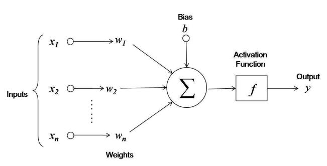
We can summarize the calculation that a neuron performs with the expression:

y = f(x1*w1 + x1*w2 + ... xn*wn + b)

where y is the output of the neuron, x1...xn are the neuron's inputs, w1...wn are the weights associated with each of its inputs, b is a bias term, and f is an activation function - a function responsible for determining the activation of the neuron's output based on a weighted sum of its inputs.

In most neural networks, the final layer of the computation that it implements is a loss function - a function that summarizes the performance of the network with respect to some input data. The lower the values produced by this loss function, the better the network is performing with respect to the task of interest. Adding the loss function to the expression above, we have:

L = loss(f(x1*w1 + x1*w2 + ... xn*wn + b), data)

where loss is the loss function itself, and data represents some data source with respect to which the loss is computed.

As we see in the diagram above, within a neural network architecture, we have a set of parameters - weights and biases - that we can tune to tweak the network's performance by changing the computation it implements. The question is: how do we tweak these parameters to achieve this improved performance?

What we need to know is: for an individual parameter, how does it contribute to the observed loss, in terms of magnitude and direction (positive or negative)? If we know this, then we can systematically adjust these parameters to reduce the loss. The way that we can express this "contribution" mathematically is in terms of the derivative of the loss with respect to the parameter in question, or the parameter's gradient.

Therefore, the problem becomes: given some computation graph and an observed loss value, how do we compute gradients for each node in the graph efficiently? An autograd engine provides exactly this functionality, via the backpropagation algorithm.

In summary, my claim is that autograd engines support neural network training by allowing us to backpropagate errors through a computation graph, thereby providing us a method to update the parameters of the network to reduce this error.

Derivative of a Simple Function

So, all we need to train a neural network is an efficient way to compute gradients through an arbitrary computation graph (a mathematical expression). We'll build up the intuition for how we can accomplish this step by step, starting with computing the derivative of a simple function:

$f (x) = 3 x^{2} - 4 x + 5$

We can implement this function in Python as:

def f(x) -> float:
    return 3*x**2 - 4*x + 5

Then, we visualize the function's behavior by generating some input values and computing the corresponding outputs:

xs = np.arange(-5, 5, 0.25)
ys = f(xs)

plt.plot(xs, ys)

The resulting plot is a simple parabola:

parabola

With some basic knowledge of calculus, we can compute the derivative of this function symbolically:

$f^{'} (x) = 6 x - 4$

Its a simple matter to implement the derivative as a function as well:

def df(x) -> float:
    return 6*x - 4

In addition to the symbolic derivative, however, we can use the definition of the derivative to compute it numerically. The definition states:

$L = {lim}_{h - > 0} \frac{f (x + h) - f (x)}{h}$

Effectively, it says:

When we change the input by a tiny amount, what is the slope (direction and magnitude) of the response of the output?

We can write a function that evaluates the derivative numerically for the function f at a provided input, for a given value of h:

def numerical(x, h: float = 0.001) -> float:
    return (f(x + h) - f(x)) / h

The quality of the estimate provided by the numerical derivative is controlled by the magnitude of the "nudge", h. We can look at how much the numerical derivative differs from the expected result provided by the symbolic derivative as a function of h:

for h in [0.1, 0.001, 0.0001, 0.00001, 0.000001]:
    print(abs(numerical(4, h=h) - df(4)))

Here, the results look like:

0.2999999999999403
0.0030000000026575435
0.00029999997821050783
2.9998357149452204e-05
2.990627763210796e-06

So, for sufficiently small values of h, the numerical derivative provides a close approximation of the symbolic derivative. We'll use this fact to check our work in the coming section when we begin work on extending this reasoning to operate on more complicated functions.

A Function with Multiple Inputs

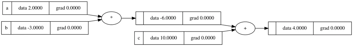
We can apply the same logic to functions with multiple inputs. Consider the function:

def f(a, b, c) -> float:
    return a*b + c

Now, because there are multiple input variables (a, b, and c) it doesn't make sense to talk about the derivative of the output of this function. Instead, we talk about the derivative of the output with respect to some input. That is, with:

$y = a * b + c$

We have three potential derivatives of interest:

$\frac{d y}{d a}, \frac{d y}{d b}, \frac{d y}{d c}$

Or, the derivative of y with respect to a, the derivative of y with respect to b, and the derivative of y with respect to c.

We can use the same method as before to approximate these derivatives numerically:

h = 0.0001

a = 2.0
b = -3.0
c = 10.0

# dy/da
(f(a + h, b, c) - f(a, b, c)) / h # approx -3.0
# dy/db
(f(a, b + h, c) - f(a, b, c)) / h # approx 2.0
# dy/dc
(f(a, b, c + h) - f(a, b, c)) / h # approx 1.0

These values match up with what we would find by evaluating this derivative symbolically.

The `Value` Object

Now that we have some intuition about what the derivative is telling us about these expressions, we can start working through the process of generalizing the ability to compute derivatives through an arbitrary computation graph.

As these expressions grow larger, or arbitrarily large, we need an automated way to maintain the computation graph that the expression represents. This way, we can construct a potentially-complicated expression and have the computation graph maintained for us automatically, which will make the task of computing gradients through the graph much simpler.

The Value object is the data structure that we'll use to maintain this computation graph. Each instance of Value represents a simple, floating-point numeric value, but it has the additional responsibility to maintain some metadata like:

The input values that were used to produce it, if any
The operation that was used to combine these input values to produce it, if any
The gradient of the output of the expression with respect to this particular node in the computation graph

The basic setup for the Value object looks like:

from __future__ import annotations

class Value:
    def __init__(self, data: float, _children: tuple[Value,...]=(), _op="", label=""):
        # the data maintained by this object
        self.data = data
        # the gradient of the output of the graph w.r.t this node
        self.grad = 0.0
        # a human-readable label for this node
        self.label = label

        # the function for computing the local gradient
        self._backward = lambda: None
        # the anscestors of this node in the graph
        self._prev = set(_children)
        # the operation used to compute this node
        self._op = _op

We can instantiate a Value object with some data:

a = Value(a, label="a")
a
# Value(data=2.0)

Aside from this, though, we can't really do anything with it yet. For instance, we can't add two Values together:

a = Value(1.0, label="a")
b = Value(2.0, label="b")
a + b
---------------------------------------------------------------------------
TypeError                                 Traceback (most recent call last)
Cell In[24], line 3
      1 a = Value(1.0, label="a")
      2 b = Value(2.0, label="b")
----> 3 a + b

TypeError: unsupported operand type(s) for +: 'Value' and 'Value'

To start working with these objects to build an expression, we'll need to implement some operations for them. We can start by implementing the __add__ method to support addition:

def __add__(self, input: float | int | Value) -> Value:
    # wrap other in a Value if not already
    other = input if isinstance(input, Value) else Value(input)

    out = Value(self.data + other.data, (self, other), "+", _next_char((self.label, other.label)))
    return out

This method supports addition with both numeric literals as well as other Value object:

a = Value(1.0, label="a")
b = Value(2.0, label="b")
c = a + b
# Value(data=3.0)

d = a + 3.0
# Value(data=4.0)

We can also implement the __radd__ function to add support for addition on the right with literals:

def __radd__(self, other: float | int | Value) -> Value:
    return self + other

Now, expressions like the following are also supported:

a = Value(1.0, label="a")
d = 3.0 + a
# Value(data=4.0)

In addition to addition, multiplication is another fundamental operation that we'll need:

def __mul__(self, input: float | int | Value) -> Value:
    other = input if isinstance(input, Value) else Value(input)

    out = Value(self.data * other.data, (self, other), "*", _next_char((self.label, other.label)))
    return out

def __rmul__(self, input: float | int | Value) -> Value:
    return self * input

The implementation is analogous to the implementation of addition. Now, we can construct expressions like the one we used as an example in the previous section:

a = Value(2.0, label="a")
b = Value(-3.0, label="b")
c = Value(10.0, label="c")

y = a*b + c
y
# Value(data=4.0)

More important than just computing the result of the expression (equivalent to the forward pass, as we'll come to see) is the fact that the Value instance y "knows" the complete computation graph that is used to compute it.

A convenient way of demonstrating this is a visual depiction of the computation graph. We won't go into the details for it here, but the repository provides some code (copied verbatim from Andrej's implementation) that is capable of displaying this graph for us:

from micrograd.util.draw import draw_dot
draw_dot(y)

simple-1

Manual Backpropagation

So far, we can build scalar-valued mathematical expressions (limited to addition and multiplication currently) and compute a "forward pass," during which the computation graph for the expression is generated automatically by our Value objects. Next, we need to start working on computing gradients throughout this graph via backpropagation.

In this section, we'll work through the backpropagation process manually for an expression to get a sense for how the calculations work. Once that is done, we'll have all of the knowledge we need to automate the calculation of gradients through the entire graph.

We'll use the slightly-more complex expression as our testbed for this exercise:

a = Value(2.0, label="a")
b = Value(-3.0, label="b")
c = Value(10.0, label="c")
e = a*b; e.label="e"
d = e + c; d.label="d"
f = Value(-2.0, label="f")
L = d*f; L.label="L"

The choice of the variable name L here is deliberate - we can think of this as representing the loss function for a neural network, and by performing backpropagation we'll be computing the contribution of each node to the output value for the loss. If we were training a neural network, this would in turn tell us how to adjust the node values (assuming they are parameters) to reduce the loss and increase the network's performance.

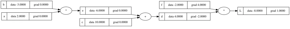
We can visualize the computation graph for this expression with the draw_dot function:

g0-1

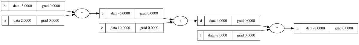
As we can see in the graph visualization, all of the gradients are currently 0.0. Our job is to fill in each of these values - we need to compute the derivative of the loss, L, with respect to each of a, b, c, etc.

At first glance, this process appears daunting. For instance, if we were begin by considering our variables left to right, how would we compute the derivative:

$\frac{d L}{d a}$

Calculus' chain rule tells us that, generally, if a variable z depends on a variable y, which in turn depends on x, then z depends on x as well, via the intermediate variable y, and that the relationship between them is:

$\frac{d z}{d x} = \frac{d z}{d y} * \frac{d y}{d x}$

Applying this same logic to our expression, we have:

$\frac{d L}{d a} = \frac{d L}{d e} * \frac{d e}{d a}$

So, we can compute the derivative of the loss, L, with respect to a given the derivative of L with respect to the intermediate variable e and the local derivative $\frac{d e}{d a}$ .

The situation is analogous for every other node in the graph, and this fact reveals a critical insight. In backpropagation, we start at the output and work backwards to compute the gradient of the output with respect to each node in the graph. We work backwards because, according to chain rule, computing the gradient for a given node is straightforward if we already know the gradient with respect to intermediate variable that is nearest to the target variable in the graph (and on the path to the output variable).

So, with our computation graph above, we'll start from the output (the right side) and work our way towards the inputs (the left side). We'll compute the derivatives symbolically, and also check our work with a numerical approximation, enabled by the following function:

def fn():
    h = 0.001

    a = Value(2.0, label="a")
    b = Value(-3.0, label="b")
    c = Value(10.0, label="c")
    e = a*b; e.label="e"
    d = e + c; d.label="d"
    f = Value(-2.0, label="f")
    L = d*f; L.label="L"
    L.data += h
    L1 = L.data

    # add some h here
    a = Value(2.0, label="a")
    b = Value(-3.0, label="b")
    c = Value(10.0, label="c")
    e = a*b; e.label="e"
    d = e + c; d.label="d"
    f = Value(-2.0, label="f")
    L = d*f; L.label="L"
    L2 = L.data

    return (L2 - L1) / h

This function allows us to "nudge" one of the values in the expression by a small amount h and observe how the output responds, according to the definition of the derivative. Without further ado, lets begin!

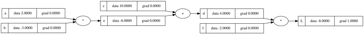
As a warmup, we can first compute the derivative of L with respect to itself, $\frac{d L}{d L}$ . Trivially, this is 1. We can check this numerically to confirm that our function is working:

    # fn()
    # ...
    L = d*f; L.label="L"
    L.data += h
    L1 = L.data
    # ...

fn()
# 1.000000000000334

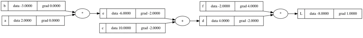
The numerical derivative confirms the symbolic one. We can now fill in this value in our computation graph, resulting in the updated graph state:

g1-1

Now the real work begins. In the next "layer" of the graph, we have the variables d and f, meaning that we can now compute $\frac{d L}{d d}$ and $\frac{d L}{d f}$ . No chain rule is required here; we can compute these derivative directly:

$\frac{d L}{d d} = f, \frac{d L}{d f} = d$

Again, we can approximate these derivatives numerically to confirm our work:

d.data += h
fn()
# -2.000000000000668

f.data += h
fn()
# 3.9999999999995595

And we can fill in these gradients accordingly:

g2-1

In the next layer, we have variables e and c. As Andrej calls out in his original lecture, if we understand this calculation (the way we calculate $\frac{d L}{d e}$ and $\frac{d L}{d c}$ ), then we understand the entire process of backpropagation. This is the first instance in which we'll need to apply the chain rule to compute the derivatives symbolically. We'll start with e with the knowledge that the same logic will apply to c.

By the chain rule, we have that:

$\frac{d L}{d e} = \frac{d L}{d d} * \frac{d d}{d e}$

We already know $\frac{d L}{d d}$ , this is just f. Furthermore, we know how to calculate $\frac{d d}{d e}$ symbolically. Therefore, we have:

$\frac{d L}{d e} & = \frac{d L}{d d} * \frac{d d}{d e} & = f * 1 & = - 2.0 * 1 & = - 2.0$

So, we expect that $\frac{d L}{d e} = - 2.0$ . We can check this numerically:

e.data += h
fn()
# -2.000000000000668

We can apply the same logic to calculate $\frac{d L}{d c} = - 2.0$ as well. It is important to take a step back and generalize what happened here. For the addition operation, the gradient for both operand values is equivalent to the gradient of the result of the operation - the addition operation merely "distributes" the gradient from the current node to the next two nodes in the graph (assuming we are working backwards).

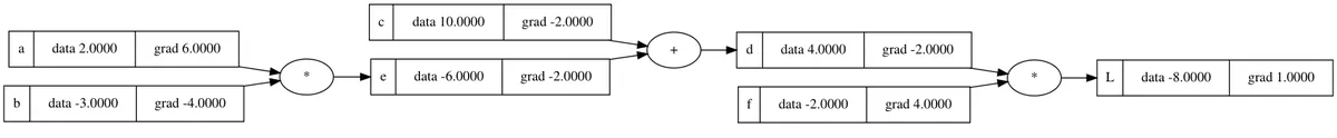
At the end of this step, the graph looks like:

g3-1

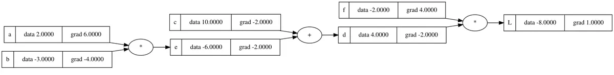
Similarly, we can apply the same logic again (chain rule) to calculate the derivatives for the final variables a and b. Taking a as our first case, the chain rule tells us that:

$\frac{d L}{d a} & = \frac{d L}{d e} * \frac{d e}{d a} & = - 2.0 * b & = - 2.0 * - 3.0 & = 6.0$

The same logic applies for b. Again, lets generalize what happened: in contrast to the addition operation, calculating the gradient for one operand value of a multiplication operation amounts to multiplying the gradient from the output value of the operation by the value of the other operand.

The final computation graph looks like:

g4-1

Implementing `.backward()`

We have now completed manual calculation of the backpropagation process for an entire computation graph. Along the way, we've built up all of the intuition we need to implement the .backward() method on our Value object, and thereby automate the process of computing gradients through the computation graph.

Our Value currently supports two operations, addition and multiplication. We saw both of these while manually computing our gradients. To add backpropagation functionality to Value, we'll fill in the _backward property of a Value instance when we construct it from an arithmetic operation. This property is a function that, when invoked, computes the gradient for the two operands of the operation, assuming that the gradient for the output is already known.

The implementation for __add__ looks like:

def __add__(self, other: float | int | Value) -> Value:
    # ...
    out = Value(self.data + other.data, (self, other), "+")

    def _backward():
        self.grad += 1.0 * out.grad
        other.grad += 1.0 * out.grad
    
    out._backward = _backward
    
    return out

Here we see what we discovered during manual backpropagation: that for addition, the gradient from the output is merely distributed to the two inputs during the backward pass. Notice that the gradients are accumulated (+=) rather than simply assigned. This is important because a single Value instance may be used in multiple sub-expressions within an expression, and the gradient for the instance must account for all of these usages.

For multiplication, we have the implementation:

def __mul__(self, other: float | int | Value) -> Value:
    # ...
    out = Value(self.data * other.data, (self, other), "*")

    def _backward():
        self.grad += other.data * out.grad
        other.grad += self.data * out.grad 
    out._backward = _backward

    return out

Now, instead of distributing the gradients, the multiplication operator results in multiplication of the gradient of the output node with the data contained within the other Value object.

Now we have a ._backward property on each node in the graph that is capable of computing the gradient for the two input operands, given the gradient of the current Value instance. Now all we need is a routine to "orchestrate" the invocation of these functions. In order to ensure that gradients are computed in the correct order - that all nodes on which a node depends for its gradient calculation have their own gradients calculated prior - we'll need an implementation of topological sort, which delivers exactly this property when executed on a directed-acyclic graph (DAG).

We won't go into detail of the implementation of the topological_sort() function here; you can check it out on GitHub if you are interested in its implementation.

With it, though, the implementation of the final .backward() method on Value is straightforward:

def backward(self) -> None:
    self.grad = 1.0
    for node in reversed(topological_sort(self)):
        node = typing.cast(Value, node)
        node._backward()

We initialize the gradient for this node to 1.0, and then invoke ._backward() on each node in a (reversed) topological sort of the computation graph.

We can check our implementation of .backward() by testing it on the same expression we used during manual backpropagation:

a = Value(2.0, label="a")
b = Value(-3.0, label="b")
c = Value(10.0, label="c")
e = a * b
e.label = "e"
d = e + c
d.label = "d"
f = Value(-2.0, label="f")
L = d * f
L.label = "L"

L.backward()
draw_dot(L)

The resulting gradients match those we calculated previously:

auto-1

Conclusion

We now have a scalar-valued autograd engine that supports addition and multiplication operations. This is a good start, but we need to add support for a few more operations, including some nonlinearities, in order to support construction of neural networks. In the next post, we'll add this support and subsequently build a tiny neural network library on top of the Value implementation that provides abstractions for neurons, layers, and multi-layer perceptrons.

#post