A Statistical Character Bigram Language Model

02 Dec, 2025

We're moving on from the lower-level details of automatic differentiation and gradient descent via backpropagation to start focusing on building models for a more sophisticated purpose: emulation of natural language. We'll build up from a simple statistical bigram model to a modern transformer-based one.

The content in this post is based on Andrej Karpathy's YouTube video. The source for his original version of makemore is available on GitHub.

All of the source code that I produced for this post is available in my makemore-and-friends repository. Specifically, the notebook bigram_stat.ipynb builds up the code with the concepts in the same order they are described below.

Making More

The goal of every model we build in the makemore family is to learn the properties of some training data such that we can generate new content that resembles this data, but may be unique from any example we encountered during training. We are specifically focused on language models, and generating natural language.

The dataset that we'll use is a small text file, names.txt, that contains English-language names. We begin by loading the input data from its file:

def load_names(path: Path) -> list[str]:
    with path.open("r") as f:
        return f.read().splitlines()
    
words = load_names(data_dir / "names.txt")

This gives us a list of the names contained within the file, with each line (name) represented as an element in the list:

print(words[:4])
# ['emma', 'olivia', 'ava', 'isabella']
len(words)
# 32033

The dataset contains just over 32,000 names.

Counting Bigrams

In our first attempt at "making more," we won't even use machine learning - we'll compute simple statistical properties of the training data and sample from the resulting statistical model.

Specifically, we'll consider character bigrams. Considering characters means that we'll look at individual characters, both when training the model and sampling from it to produce new data. This is in contrast to more sophisticated models that might consider higher-level structure, like words. Character bigrams are pairs of two characters; our bigram language model will consider just two characters at a time, collecting statistics for the next character based only on the character that immediately precedes it.

We can look at the bigrams provided by a single word:

w = words[0]
for l, r in zip(w, w[1:]):
    print((l, r))

This produces the output:

('e', 'm')
('m', 'm')
('m', 'a')

When counting all of the bigrams across the entire dataset, we'll want to track two additional pieces of information:

When a character appears at the start of a word
When a character appears at the end of the word

To implement this, we'll introduce a special token, ., which we will inject during the counting process. We can add this injection logic to the loop from before:

w = ["."] + list(words[0]) + ["."]
for l, r in zip(w, w[1:]):
    print((l, r))

Now we get the bigrams:

('.', 'e')
('e', 'm')
('m', 'm')
('m', 'a')
('a', '.')

Applying this same logic to the entire dataset, we can count the number of occurrences of all character bigrams:

TOKEN_DOT = "."

bigram_counts = {}
for w in words:
    chs = [TOKEN_DOT] + list(w) + [TOKEN_DOT]
    for l, r in zip(chs, chs[1:]):
        bigram = (l, r)
        bigram_counts[bigram] = bigram_counts.get(bigram, 0) + 1

We can then look at the most common bigrams:

sorted(bigram_counts.items(), key=lambda p: p[1], reverse=True)[:10]

The results reveal the 10 most common character bigrams for the entire dataset:

[(('n', '.'), 6763),
 (('a', '.'), 6640),
 (('a', 'n'), 5438),
 (('.', 'a'), 4410),
 (('e', '.'), 3983),
 (('a', 'r'), 3264),
 (('e', 'l'), 3248),
 (('r', 'i'), 3033),
 (('n', 'a'), 2977),
 (('.', 'k'), 2963)]

The most common bigram indicates that the character n terminates a word 6,763 times throughout this dataset. Similar, a followed by . (the end of the word) is the second most common bigram in this dataset, with 6,640 occurrences.

Converting to a Tensor Representation

This dictionary-based representation of the bigram counts data structure is comprehensible but inefficient. We can do better by converting to a tensor representation using a Tensor from pytorch.

The first step towards implementing this representation is to support mapping a character to an integer (and back) - we need this to translate between characters and the indices in the tensor that represent them. We achieve this by identifying all of the unique characters in the dataset (our vocabulary), and mapping them to an index based on an alphabetical sort. We insert the special . token at index 0.

Finally, we reverse this mapping such that we can map from character to index and from index to character, bidirectionally.

# LUT construction
chars = sorted(list(set("".join(words))))

# string-to-index
stoi = {c: i+1 for i, c in enumerate(chars)}
stoi[TOKEN_DOT] = 0

# index to string
itos = {i: c for c, i in stoi.items()}

With these mappings, we can now update our bigram-counting logic to store counts in a Tensor.

import torch

# 26 characters + 1 special token
ALPHABET_SIZE = 27 

# initialize counts to 0
N = torch.zeros((ALPHABET_SIZE, ALPHABET_SIZE), dtype=torch.int32)

for w in words:
    chs = [TOKEN_DOT] + list(w) + [TOKEN_DOT]
    for l, r in zip(chs, chs[1:]):
        il = stoi[l]
        ir = stoi[r]
        N[il, ir] += 1

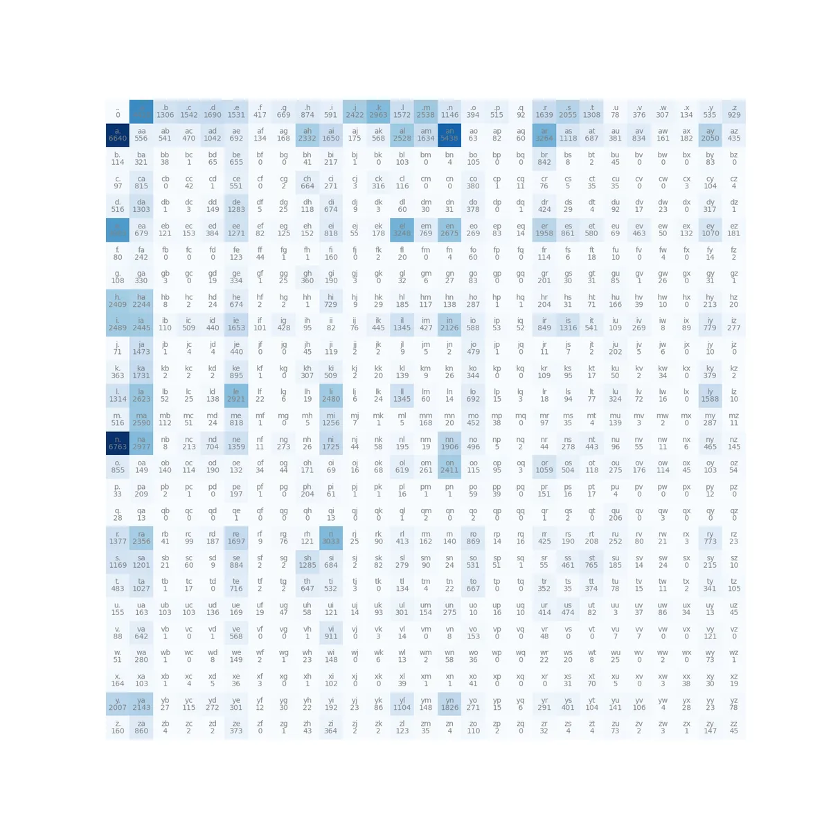
Here, the first character in the bigram appears as a row in the tensor, and the second characters appears as a column. So, a value of 13 at index (1, 2) indicates that the bigram (a, b) appears in the dataset 13 times.

We can use the following code to visualize the entire counts matrix:

import matplotlib.pyplot as plt
%matplotlib inline

plt.figure(figsize=(16, 16))
plt.imshow(N, cmap="Blues")
for i in range(ALPHABET_SIZE):
    for j in range(ALPHABET_SIZE):
        chstr = itos[i] + itos[j]
        plt.text(j, i, chstr, ha="center", va="bottom", color="gray")
        plt.text(j, i, str(N[i, j].item()), ha="center", va="top", color="gray")

plt.axis("off")

The resulting figure summarizes the bigram frequency across the entire dataset:

matrix

Sampling from the Model

Now that we've "learned" statistical properties of the dataset in the form of bigram counts, we can sample from the model to produce new content from this same distribution.

We'll use a pytorch Generator to make sampling results reproducible across invocations. In the code below, we create a Generator, use it to generate some random values on [0, 1), and then normalize these values to a probability distribution:

g = torch.Generator().manual_seed(1337)
p = torch.rand(3, generator=g)
p = p / p.sum()
p
# tensor([0.0654, 0.4140, 0.5205])

We can then use torch.multinomial to sample from this probability distribution. This allows us to get an index into the tensor based on the probability assigned to that index - i.e. sample from the multinomial distribution p.

samples = torch.multinomial(p, num_samples=32, replacement=True, generator=g)
samples
# tensor([1, 1, 2, 1, 2, 1, 2, 2, 1, 2, 2, 2, 2, 2, 2, 2, 1, 1, 2, 2, 1, 2, 2, 1, 1, 2, 1, 1, 2, 2, 1, 1])

We can manually verify that the distribution of the samples we collected with torch.multinomial is close to our expectations based on the original probabilities:

prop_0 = (samples == 0.0).sum().item() / len(samples)
prop_1 = (samples == 1.0).sum().item() / len(samples)
prop_2 = (samples == 2.0).sum().item() / len(samples)

props = [prop_0, prop_1, prop_2]
props
# [0.0, 0.4375, 0.5625]

We can use this same logic to sample a single word from the bigram model. The one optimization we'll make along the way is to pre-normalize the rows of the tensor such that we don't need to repeatedly re-compute the probability distribution. With pytorch, it is a simple matter to perform these row-wise operations, dividing each element in a particular row by the sum along that row.

# create a copy of bigram counts
P = N.float()
# normalize to probability distribution along rows
P /= P.sum(1, keepdim=True)

In Andrej's original video he includes a great discussion of broadcasting semantics for PyTorch tensors. It is definitely worth a watch if there is any confusion as to why the division operation in the snippet above produces the output we want - I certainly gained some useful intuition from his explanation.

Now, each row in the tensor is a probability distribution that corresponds to a single character. For that character, it provides the probability that it is immediately followed by every other character in the vocabulary.

Once we have computed the probability distribution for each character, we can write the following logic to sample a single word from the model:

def sample_one(model: torch.Tensor, g: torch.Generator) -> str:
    """Sample a single word from the model."""
    word = ""

    ix = 0 # 0 is the index of the start token '.'
    while True:
        # sample an index from the distribution
        ix = torch.multinomial(model[ix, :].float(), num_samples=1, generator=g).item()

        # check if this is the stop token
        if ix == 0:
            return word
        
        # add the character to the growing word
        word += itos[ix]

And we can wrap some additional logic around this to sample multiple words:

def sample(model: torch.Tensor, k: int = 1, seed: int = 1337):
    """Sample k words from the model."""
    g = torch.Generator().manual_seed(seed)
    return [sample_one(model, g) for _ in range(k)]

We can then invoke this function to draw some samples:

samples = sample(N, k=8)
samples

These samples look like:

'gun',
'kaneliy',
'dy',
'exylell',
'eleleahmariss',
'modarrinam',
'rn',
'vybeartosay'

As names, these samples leave something to be desired. The underlying issue is that character bigrams produce a simple model of the training data, capturing only small, local structure. In future posts in this series we'll construct more sophisticated models that produce names that are subjectively higher in quality (i.e. realism).

Loss Function

In addition to subjectively evaluating the model's quality by sampling from it, we'd like some means of computing its quality automatically. We need a loss function - a function that takes as input our model and some data and produces a single number that summarizes the model's quality with respect to that data. Typically, loss functions follow the convention that higher values are worse while lower values (closer to 0) are better.

We can start constructing our loss function by observing that we can calculate the probability that the model assigns to each bigram in the dataset:

w = words[0]
chs = [TOKEN_DOT] + list(w) + [TOKEN_DOT]
for l, r in zip(chs, chs[1:]):
    ix0, ix1 = stoi[l], stoi[r]
    # probability that this bigram appears
    prob = model[ix0, ix1]

Because we treat each of these events (bigrams) as independent, we can compute the likelihood - an overall measure of how well our model explains observed data - as the product of these individual probabilities for each bigram.

likelihood = 1.0
for w in words:
    chs = [TOKEN_DOT] + list(w) + [TOKEN_DOT]
    for l, r in zip(chs, chs[1:]):
        ix0, ix1 = stoi[l], stoi[r]
        likelihood *= model[ix0, ix1]

We run into a problem with calculation of the likelihood, however, because repeated multiplication by values between 0 and 1 quickly drives the magnitude of the likelihood to be vanishingly small. After some number of calculations like this, we'll lose all precision as we reach the limits of the binary representation of floating point numbers.

To get around this, we'll work with the log-likelihood. For our purposes, an important property of the logarithm is that it is a monotonically-increasing function:

log

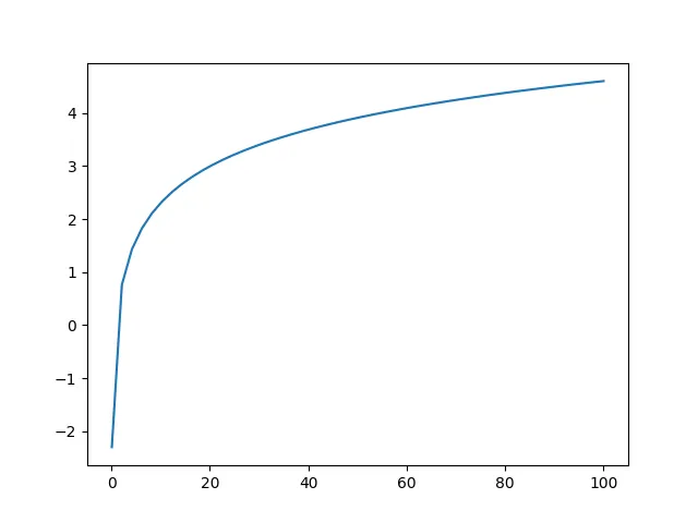
Therefore, our transformation is valid: maximizing the log-likelihood is equivalent to maximizing the likelihood. Furthermore, the logarithm function has useful property that

$\log (a * b * c) = \log (a) + \log (b) + \log (c)$

implying that we can compute the log-likelihood as a sum of the logarithm of the individual bigram probabilities assigned by our model.

log_likelihood = 0.0
for w in words:
    chs = [TOKEN_DOT] + list(w) + [TOKEN_DOT]
    for l, r in zip(chs, chs[1:]):
        ix0, ix1 = stoi[l], stoi[r]
        log_likelihood += torch.log(model[ix0, ix1]).item()

We said above that loss functions have the property that "lower is better," but currently we are talking about maximizing the likelihood. We can invert this value to produce the negative log-likelihood, which now fits the expected semantics of a loss function.

log_likelihood = 0.0
for w in data:
    chs = [TOKEN_DOT] + list(w) + [TOKEN_DOT]
    for l, r in zip(chs, chs[1:]):
        ix0, ix1 = stoi[l], stoi[r]
        log_likelihood += torch.log(model[ix0, ix1]).item()

# invert to get negative log-likelihood
nll = -log_likelihood

We perform one final transformation to compute the mean negative log-likelihood across all of the bigrams against which we are evaluating our loss. Now, the final value represents the average loss across every evaluation example, rather than the sum of these example-level losses.

The final loss function looks like:

def loss(model: torch.Tensor, data: list[str]) -> float:
    """Compute loss with respect to the given data."""
    # the number of bigrams
    n = 0

    log_likelihood = 0.0
    for w in data:
        chs = [TOKEN_DOT] + list(w) + [TOKEN_DOT]
        for l, r in zip(chs, chs[1:]):
            ix0, ix1 = stoi[l], stoi[r]
            log_likelihood += torch.log(model[ix0, ix1]).item()
            n += 1

    # invert to get negative log-likelihood
    nll = -log_likelihood
    # compute mean of negative log-likelihood
    return nll / n

We can now use this to summarize the quality of our model:

loss(P, words)
# 2.4540144946949742

Our loss with respect to the entire training dataset is ~2.45.

Model Smoothing

Our model has a subtle issue. Consider a case where we compute the loss with respect to a word that contains a bigram that was never encountered in the training dataset:

loss(P, ["andrejq"])
# inf

The resulting loss is infinite. This occurs because the probability assigned by our model to the bigram jq is 0.0:

P[stoi["j"], stoi["q"]]
# tensor(0.)

Then, when we compute the logarithm of 0, we get -inf, because the domain of the logarithm function is the set of all positive real numbers:

torch.log(P[stoi["j"], stoi["q"]]).item()
# -inf

This in turn causes the aggregate negative log-likelihood and the average log-likelihood to remain fixed at inf.

We can apply a model smoothing technique to address this issue via a simple mechanism: fake counts. Effectively, we add a fixed value (like 1) to the counts for each bigram to make the situation that we just encountered impossible. We can inject thes fake counts while computing bigram probabilities from the raw counts tensor:

P = (N+1).float()
# ...

Now, there is always some nonzero probability that a particular bigram might be generated by our model, though these probabilities should remain quite small for bigrams that were not present in the training set.

Now we can recompute the loss for this example without experiencing an infinite loss:

loss(P, ["andrejq"])
# 3.4834019988775253

Its also important to note, however, that applying smoothing does increase our overall loss, albeit not significantly:

loss(P, words)
# 2.4545768249521656

This is about 0.0006 higher than the loss we computed prior to applying smoothing.

Conclusions and Next Steps

We've trained and evaluated a simple statistical language model using character bigrams. Along the way, we discussed the concept of a loss function as a means of assessing model quality. For now, this loss function allows us to evaluate the performance impact of manual tweaks to our model, and we'll see some of this at work in the next post. However, following that, we'll re-implement the character bigram model in a machine learning paradigm (rather than a statistical one); there, the loss function will provide a means of automatically updating the model's parameters to improve its performance.

#post