More Autograd: Arithmetic Operations, Nonlinearities, and a Simple Neural Network Library
In my previous post, we built a scalar-valued autograd engine that supports addition and multiplication operations. Here, we'll continue to build on this implementation, adding support for additional arithmetic operations (e.g. subtraction, division), writing the nonlinear functions we need to serve as activations, and finally building a little neural network library on top of the engine.
Again, credit for this implementation goes to Andrej Karpathy and his original video on the topic here. Andrej's source code for micrograd is also available on GitHub.
My implementation, which cleans a few things up an builds on Andrej's, is also on GitHub; the notebook that aligns with this tutorial is here.
New Arithmetic Operations
At the end of the previous post, the complete implementation of the Value object, the core of the autograd engine, is just a few lines of code:
from __future__ import annotations
import typing
from micrograd.util.graph import topological_sort


class Value:
    def __init__(
        self,
        data: float | int,
        _children: tuple[Value, ...] = (),
        _op="",
        label="",
    ):
        # the data maintained by this object
        self.data = data
        # the gradient of the output of the graph w.r.t this node
        self.grad = 0.0
        # a human-readable label for this node
        self.label = label

        # the function for computing the local gradient
        self._backward = lambda: None
        # the ancestors of this node in the graph
        self._prev = set(_children)
        # the operation used to compute this node
        self._op = _op

    def __repr__(self) -> str:
        return f"Value(data={self.data})"

    def __add__(self, other: float | int | Value) -> Value:
        # wrap other in a Value if not already
        other = other if isinstance(other, Value) else Value(other)

        out = Value(self.data + other.data, (self, other), "+")

        def _backward():
            self.grad += 1.0 * out.grad
            other.grad += 1.0 * out.grad

        out._backward = _backward

        return out

    def __radd__(self, other: float | int | Value) -> Value:
        return self + other

    def __mul__(self, other: float | int | Value) -> Value:
        other = other if isinstance(other, Value) else Value(other)

        out = Value(self.data * other.data, (self, other), "*")

        def _backward():
            self.grad += other.data * out.grad
            other.grad += self.data * out.grad

        out._backward = _backward

        return out

    def __rmul__(self, other: float | int | Value) -> Value:
        return self * other

    def backward(self) -> None:
        self.grad = 1.0
        for node in reversed(topological_sort(self)):
            node = typing.cast(Value, node)
            node._backward()
We can use this class to build expressions consisting of addition and multiplication operations (with other Values or scalars), and critically we can run the backward pass the the resulting computation graph to compute gradients.
To build more diverse expressions, and to support some of the more sophisticated operations we'll need to implement a neural network library, we'll need to implement a few more arithmetic operators, namely negation, subtraction, exponentiation, and division.
For most of these, we won't need to build them from scratch; instead we'll construct these from the existing arithmetic operations we've already implemented. This saves us the trouble of having to compute the derivative for the backward pass.
Negation is the simplest; we can express this as multiplication with -1:
def __neg__(self) -> Value:
    return self * -1
Again, no other logic is necessary here. Our implementation of __mul__ kicks in and handles both the forward and backward passes. Now we can:
a = Value(2.0, label="a")
b = -a
b
# Value(data=-2.0)
Now that we can negate Values, we can implement subtraction:
def __sub__(self, other: Value | int | float) -> Value:
    return self + (-other)
Now we can perform subtraction with another Value instance:
a = Value(2.0, label="a")
b = Value(3.0, label="b")
c = a - b
c
# Value(data=-1.0)
or with a primitive type:
a = Value(2.0, label="a")
c = a - 3.0
c
# Value(data=-1.0)
Exponentiation, the __pow__ operator, is a different story. We could implement this as repeated multiplication, but that would be terribly inefficient. We'll implement __pow__ from scratch to avoid this inefficiency. We'll also only add support for exponentiation by a primitive type (as opposed to another Value instance) to reduce the complexity of the backward pass.
The forward pass is easy, we just exponentiate the data property of the self instance by the input:
out = Value(self.data**other, (self,), f"**{other}")
The backward pass requires the derivative of this simple exponential expression. Calculus' power rule states:
We combine this with the chain rule, multiplying this result by the gradient of the downstream node in the graph, to get the final gradient calculation:
def _backward():
    self.grad += other * (self.data ** (other - 1.0)) * out.grad
We can put this all together now to implement the __pow__ operator:
def __pow__(self, other: int | float) -> Value:
    assert isinstance(other, (int, float)), "broken precondition"

    out = Value(self.data**other, (self,), f"**{other}")

    def _backward():
        self.grad += other * (self.data ** (other - 1.0)) * out.grad

    out._backward = _backward

    return out
And now we can perform exponentiation by primitive types:
a = Value(2.0, label="a")
b = a**2.0
b
# Value(data=4.0)
Finally, with exponentiation in hand, we can implement division as a composition of existing operators. We have that:
We use this equality to implement division in terms of multiplication and exponentiation:
def __truediv__(self, other: float | int | Value) -> Value:
    return self * other**-1
This is all that is required to add support for division by both Values and primitives:
a = Value(2.0, label="a")
b = Value(4.0, label="b")
c = a / b
c
# Value(data=0.5)
Nonlinearities
In my previous post, I used the following diagram to illustrate the mathematical neuron that serves as the building block of modern neural networks:
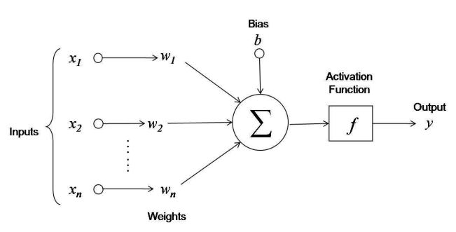
Translating this diagram to an equation, the activation of the neuron (y) as a function of inputs (x1...xn), weights (w1...wn) and a bias term (b) is expressed as:
Currently, our autograd engine supports nearly all of the operations necessary to implement this expression. We have both addition and multiplication, which are all that is required to implement the "weighted sum" that appears as input to the activation function f. All that remains, therefore, is the activation function itself.
The activation function is applied to the intermediate result produced by the neuron to introduce non-linearity; this enables the network to learn complex patterns. If the network were a linear function, it would be incapable of learning the complex patterns that underlie many of the tasks for which we rely on neural networks today, including image and speech recognition.
There are multiple classes of non-linear functions that may be used as activations in neural networks, each of which may contain multiple functions. For our implementation, we'll focus on just two: hyperbolic tangent (tanh) and rectified linear unit (ReLU).
tanh
The hyperbolic tangent function, tanh, looks like this:
The implementation in Python is straightforward:
def tanh(x) -> float:
    return (math.exp(x) - math.exp(-x)) / (math.exp(x) + math.exp(-x))
We can plot this function to get a sense for how it transforms its inputs:
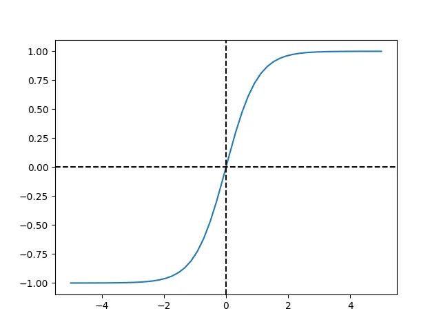
tanh maps inputs onto the range (-1.0 1.0). Large negative or large positive values approach -1.0 and 1.0, respectively.
We can drop the logic from our Python implementation of the hyperbolic tangent into our tanh method to produce the forward pass:
def tanh(self) -> Value:
    x = self.data
    t = (math.exp(x) - math.exp(-x)) / (math.exp(x) + math.exp(-x))
    out = Value(t, (self,), "tanh")
We save the intermediate value t as a variable because we'll need it for the derivative.
While we could derive it ourself (given sufficient knowledge from high school calculus), the helpful activation function Wikipedia article lists the derivative of tanh as:
Therefore, our implementation of _backward, with the addition of the chain rule, becomes:
def _backward():
    self.grad += (1 - t**2) * out.grad
We can combine these elements to produce our final implementation of tanh:
def tanh(self) -> Value:
    x = self.data
    t = (math.exp(2 * x) - 1) / (math.exp(2 * x) + 1)
    out = Value(t, (self,), "tanh")

    def _backward():
        self.grad += (1 - t**2) * out.grad

    out._backward = _backward
    return out
Now, we can apply the hyperbolic tangent activation to Value instances to compute both forward and backward passes:
# forward
a = Value(2.0, label="a")
b = a.tanh()
b # Value(data=0.964027580075817)

# backward
b.backward()
a.grad # 0.0706508248531642
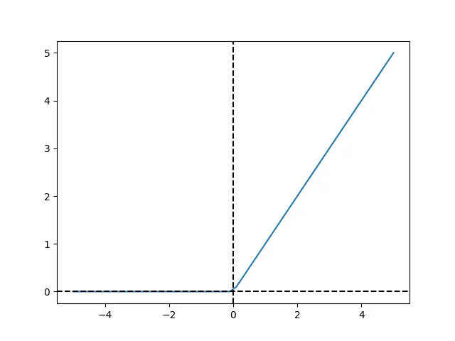
ReLU
The rectified linear unit, or ReLU is the technical name for a very simple function: it is merely the nonnegative part of its argument.
The Python implementation is a simple conditional:
def relu(x: float) -> float:
    return 0.0 if x <= 0.0 else x
As before, we can plot ReLU to get a sense for how it operates:
As was the case with hyperbolic tangent, we can drop our implementation of relu into our Value implementation to compute the forward pass:
def relu(self) -> Value:
    x = self.data
    t = 0.0 if x <= 0.0 else x
    out = Value(t, (self,), "relu")
The derivative of ReLU is given by:
This lends itself to another trivial implementation in Python:
def _backward():
    self.grad += (0.0 if x < 0.0 else 1.0) * out.grad
Bringing it all together we have:
def relu(self) -> Value:
    x = self.data
    t = 0.0 if x <= 0.0 else x
    out = Value(t, (self,), "relu")

    def _backward():
        self.grad += (0.0 if x < 0.0 else 1.0) * out.grad

    out._backward = _backward

    return out
And as was the case before for tanh we can now apply the relu activation to Value instances to compute both forward and backward passes:
# forward
a = Value(2.0, label="a")
b = a.relu()
b # Value(data=2.0)

# backward
b.backward()
a.grad # 1.0
A Simple Neural Network Library
We now have an implementation of the Value class that we can implement the abstractions necessary to build a neural network from scratch. We begin with the lowest-level primitive, the Neuron, but before we get there, we'll implement a simple base class that provides some common methods that will be exposed by all of our neural network abstractions.
class Module:
    def __init__(self) -> None:
        pass

    def parameters(self) -> list[Value]:
        return []

    def zero_grad(self) -> None:
        for p in self.parameters():
            p.grad = 0
The Module class provides logic for retrieving all of the tunable parameters for the abstraction that overrides it. It also provides a function that zeroes out all of the gradients for these parameters; this is a critical step in neural network training, as we'll see later.
Now, we can implement the Neuron abstraction, inheriting from Module. The constructor initializes the parameters (weights and bias term) of the neuron randomly with Value instances. We also provide some logic to support several different activation functions in the Neuron implementation:
class Neuron(Module):
    def __init__(self, nin: int, activation: str = "relu") -> None:
        self.w = [Value(random.uniform(-1, 1)) for _ in range(nin)]
        self.b = Value(random.uniform(-1, 1))

        match activation:
            case "relu":
                self.activation = lambda v: v.relu()
            case "tanh":
                self.activation = lambda v: v.tanh()
            case "none":
                self.activation = lambda v: v
            case _:
                raise ValueError(f"unknown activation '{activation}'")
The __call__ method implements the forward pass, computing the expression that we saw above at the start of the nonlinearies section:
def __call__(self, x: list[float] | list[int] | list[Value]) -> Value:
    # input may be wrapped in Value already, or cast here
    _x = typing.cast(
        list[Value], x if isinstance(x[0], Value) else [Value(v) for v in x] # type: ignore
    )
    # w * x + b
    weighted_sum = sum((wi * xi for wi, xi in zip(self.w, _x)), self.b)
    # apply the activation
    return self.activation(weighted_sum)
We support cases in which the input is a list of primitive types (float, int) as well as the case in which these primitives are already wrapped in Value objects. Finally, we provide a simple method to retrieve all of the parameters of the Neuron:
def parameters(self) -> list[Value]:
    return self.w + [self.b]
Now we can take this Neuron for a spin.
n = Neuron(4)

# forward
y = n([1.0, 2.0, 3.0, 4.0])
y # Value(data=1.3208788625187333)

# backward
y.backward()
print([p.grad for p in n.parameters()])
# [1.0, 2.0, 3.0, 4.0, 1.0]
Performing the backward pass populated the gradients for each of the neuron's parameters, as expected.
To compose a collection of Neurons in a single layer, we implement the Layer abstraction:
class Layer(Module):
    def __init__(self, nin: int, nout: int, **kwargs) -> None:
        self.neurons = [Neuron(nin, **kwargs) for _ in range(nout)]

    def __call__(self, x: list[float] | list[Value]) -> list[Value] | Value:
        outs = [n(x) for n in self.neurons]
        return outs[0] if len(outs) == 1 else outs

    def parameters(self) -> list[Value]:
        return [p for neuron in self.neurons for p in neuron.parameters()]
In the constructor, the nout parameter defines the number of neurons in the layer, while the nin parameter defines the number of inputs to each neuron in the layer. That is, this is a fully connected layer in which all inputs to the layer are connected to all neurons within the layer.
The forward pass for the layer merely computes the forward pass for each neuron in the layer. We collapse the output to a single Value instance if the layer has a single-dimensional output, otherwise a list of Values are returned.
l = Layer(4, 1)

# forward pass
y = l([1.0, 2.0, 3.0, 4.0])
y # Value(data=0.0)

# backward pass
y.backward()
print([p.grad for p in l.parameters()])
# [1.0, 2.0, 3.0, 4.0, 1.0]
This is the expected output because we specified nout=1 in this simple example - we only have one neuron in the layer.
Finally, we can stack multiple layers on top of one another with the multi-layer perceptron, MLP, abstraction:
class MLP(Module):
    def __init__(self, nin: int, nouts: list[int]) -> None:
        sz = [nin] + nouts
        self.layers = [
            Layer(
                sz[i],
                sz[i + 1],
                activation="none" if i == len(nouts) - 1 else "relu",
            )
            for i in range(len(nouts))
        ]

    def __call__(self, x: list[float] | list[Value]) -> Value:
        _x = x if isinstance(x[0], Value) else [Value(v) for v in x]
        _x = typing.cast(list[Value], _x)

        for layer in self.layers:
            r = layer(_x)
            _x = [r] if isinstance(r, Value) else r

        assert len(_x) == 1, "broken invariant"
        return _x[0]

    def parameters(self) -> list[Value]:
        return [p for layer in self.layers for p in layer.parameters()]
The nouts parameter is now a list the specifies the size of each layer in the network. In the constructor, we specify that each layer in the network apart from the final layer has a nonlinear activation applies to the output of the neuron.
In the __call__ method, we iterate through the layers of the MLP, computing the forward pass through each. Because each layer expects a list of inputs rather than a single value, we perform some wrapping of the output with each iteration.
We can now perform forward and backward passes with a full multi-layer perceptron:
m = MLP(2, [16, 16, 1])
len(m.parameters()) # 337

# forward pass
y = m([1.0, 2.0])

# backward pass
y.backward()
This defines a three-layer MLP. The input layer has 16 neurons, each of which accepts inputs of dimension 2. The next layer is another layer of 16 neurons, fully-connected to all neurons in the previous layer. The final layer is out output layer containing a single neuron; an activation is not applied to the output of the neuron in this layer.
Taking it for a Spin
All that remains is to take this little neural network library for a spin on a real machine learning problem. To do this, I built a simple demo notebook that builds on Andrej's original.
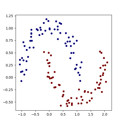
We start by building a simple dataset using sklearn's make_moons function:
from sklearn.datasets import make_moons

X, y = make_moons(n_samples=128, noise=0.1)
# make y be -1 or 1
y = y * 2 - 1

# visualize in 2D
plt.figure(figsize=(5, 5))
plt.scatter(X[:, 0], X[:, 1], c=y, s=20, cmap="jet")
Now, we can define our model with the help of our neural network library:
from micrograd.nn import MLP
model = MLP(2, [16, 16, 1])
len(model.parameters()) # 337
Now we need to define a loss function that evaluates the quality of our model with a single number. We'll discuss loss functions in more detail in a separate post. Here, we use SVM max-margin loss with L2 regularization. However, its enough to understand that the loss function accepts our model's predictions and the training data as input, assesses the current quality of our model's predictions, and outputs this "total loss" value as a Value instance, meaning that we can invoke its .backward() method to perform backpropagation and update the gradients throughout our network.
# define loss function
def loss(batch_size: int | None = None) -> tuple[Value, float]:
    # inline DataLoader
    if batch_size is None:
        Xb, yb = X, y
    else:
        ri = np.random.permutation(X.shape[0])[:batch_size]
        Xb, yb = X[ri], y[ri]
    inputs = [list(map(Value, xrow)) for xrow in Xb]

    # forward the model to get scores
    scores = list(map(model, inputs))

    # SVM "max-margin" loss (tanh instead of relu)
    losses = [(1 + -yi * scorei).relu() for yi, scorei in zip(yb, scores)]
    data_loss = sum(losses) * (1.0 / len(losses))

    # L2 regularization
    alpha = 1e-4
    reg_loss = alpha * sum((p * p for p in model.parameters()))

    # total loss
    total_loss = data_loss + reg_loss
    assert isinstance(total_loss, Value)

    # also get accuracy
    accuracy = [(yi > 0) == (scorei.data > 0) for yi, scorei in zip(yb, scores)]
    return total_loss, sum(accuracy) / len(accuracy)
We can use this loss() implementation to assess the current loss value, as well as the accuracy of our model:
total_loss, acc = loss()
print(f"total loss = {total_loss.data}, accuracy = {acc}")
# total loss = 1.1679593964096144, accuracy = 0.5
Prior to training, we achieve 50% accuracy.
Now we can conduct the optimization process. A single iteration of this process has just a few key steps:
- Compute the loss by comparing our model's predictions to the desired outputs
- Zero the gradients for all parameters in the network, and subsequently compute the backward pass to propagate these gradients
- Use these gradients to update the parameters in the network, according to some schedule; here, we use stochastic gradient descent with learning rate decay
We repeat this simple procedure for multiple iterations, optimizing the network's parameters to produce outputs that are closer and closer to the desired values.
N_EPOCHS = 32

# optimization
for k in range(N_EPOCHS):
    # forward
    total_loss, acc = loss()

    # backward
    model.zero_grad()
    total_loss.backward()

    # update (sgd) with learning rate decay
    learning_rate = 1.0 - 0.9 * k / 100
    for p in model.parameters():
        p.data -= learning_rate * p.grad

    if k % 2 == 0:
        print(f"step {k} loss {total_loss.data}, accuracy {acc*100}%")
At the end of training, we can compute the final loss and accuracy for the model:
total_loss, acc = loss()
print(f"loss {total_loss.data}, accuracy {acc*100}%")
# loss 0.10626970523128114, accuracy 97.65625%
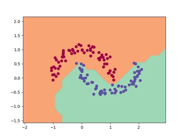
After just 32 iterations, the model achieves impressive accuracy, albeit on this relatively simple task. We can also visualize the decision boundary learned by our network:
Wrap-up
In this two-part sequence, we built from a working knowledge of calculus to a tiny neural network library that is capable of solving real machine learning problems.
I first learned neural networks in Carnegie Mellon's introduction to machine learning course. Though I was taught by world-class instructors, and I built a reasonably-complicated neural network from scratch, I still found them a bit mysterious, and therefore a bit scary because I didn't truly understand them. I think this was because we were taught neural networks in a way that lends itself to computational efficiency - via vectorized operations with matrix / vector multiplication. We also computed derivatives manually for each layer, rather than relying on a general-purpose autograd engine to handle these calculations for us.
It is only after working through this simple implementation with micrograd, narrating each step of the design and implementation, that I've realized the methods - the math and the software abstractions - underlying these extremely capable systems is truly simple and elegant. I hope these two posts help you reach a similar conclusion.
Finally, thanks again to Andrej Karpathy for building the original micrograd, and for documenting it so coherently in his video lecture.